Chapter 19: Heteroskedasticity
In this part of the book, we are systematically investigating failures to conform to the requirements of the classical econometric model. We focus in this chapter on the requirement that the tickets in the box for each draw are identically distributed across every X variable. When this condition holds, the error terms are homoskedastic, which means the errors have the same scatter regardless of the value of X. When the scatter of the errors is different, varying depending on the value of one or more of the independent variables, the error terms are heteroskedastic.
Heteroskedasticity has serious consequences for the OLS estimator. Although the OLS estimator remains unbiased, the estimated SE is wrong. Because of this, confidence intervals and hypotheses tests cannot be relied on. In addition, the OLS estimator is no longer BLUE. If the form of the heteroskedasticity is known, it can be corrected (via appropriate transformation of the data) and the resulting estimator, generalized least squares (GLS), can be shown to be BLUE. This chapter is devoted to explaining these points.
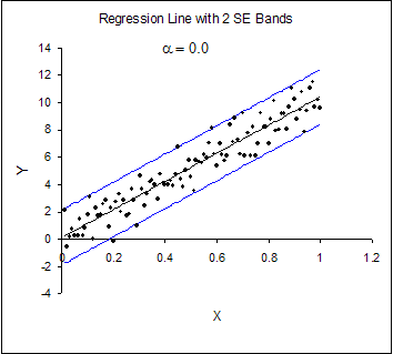
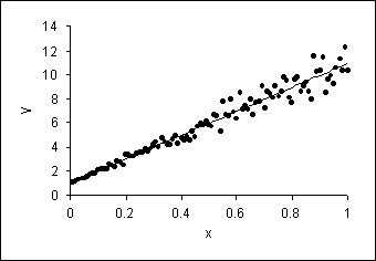
Heteroskedasticity can best be understood visually. Figure 19.1.1 depicts a classic picture of a homoskedastic situation. We have drawn a regression line estimated via OLS in a simple, bivariate model. The vertical spread of the data around the predicted line appears to be fairly constant as X changes. In contrast, Figure 19.1.2 shows the same model with heteroskedasticity. The vertical spread of the data around the predicted line is clearly increasing as X increases.

Figure 19.1.1. Homoskedasticity in a Simple, Bivariate Model.
One of the most difficult parts of handling heteroskedasticity is that it
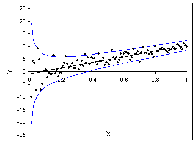
can take many different forms. Figure 19.1.3 shows another example of heteroskedasticity.
In this case, the spread of the errors is large for small values of X
and then gets smaller as X rises. If the spread of the errors is
not constant across the X values, heteroskedasticity is present.

Figure 19.1.2. Heteroskedasticity in a Simple, Bivariate Model.

Figure 19.1.3. Another Form of Heteroskedasticity
This chapter is organized around four basic issues:
• Understanding the violation itself
• Appreciating the consequences of the violation
• Diagnosing the presence of the violation
• Correcting the problem.
The next two sections (19.2 and 19.3) describe heteroskedasticity and its
consequences in two simple, contrived examples. Although heteroskedasticity
can sometimes be identified by eye, Section 19.4 presents a formal hypothesis
test to detect heteroskedasticity. Section 19.5 describes the most common
way in which econometricians handle the problem of heteroskedasticity –
using a modified computation of the estimated SE that yields correct reported
SEs. Section 19.6 discusses a more aggressive method for dealing with heteroskedasticity
comparable to the approaches commonly employed in dealing with autocorrelation
in which data transformation is applied to obtain the best linear unbiased
estimator. Finally, Section 19.7 offers an extended discussion of heteroskedasticity
in an actual data set.
Excel Workbooks
BPSampDist.xls
Het.xls
HetGLS.xls
HetRobustSE.xls
WagesOct97.xls